

LLM Cost Optimization: A Practical Engineering Playbook
19 min read

Route routine requests to cheaper models, enable prompt caching on repeated system prompts, and switch eligible workloads to batch APIs. That combination, according to practitioner benchmarks, typically delivers the largest dollar savings for the least engineering effort — often cutting inference spend by 50–90% on the requests it touches. Here is the prioritized checklist to hand your team today:
- Model routing (owner: ML/platform engineer, validate in 1 day): classify requests by complexity and send simple tasks to a cheaper model tier. Expected savings on routed requests can be significant.
- Prompt caching (owner: API integration engineer, validate in 1 hour): cache static system prompts at the provider level. Expected savings: up to 90% on repeated input tokens.
- Batch API (owner: DevOps, validate in 1 day): move non-latency-sensitive workloads to provider batch endpoints. Expected savings of about half off standard pricing.
- Cost tagging and attribution (owner: platform/FinOps engineer, validate in 1 week): tag every request with team, feature, and use-case metadata so you can measure the ROI of each lever above.
- Pre-flight token estimation (owner: backend engineer, validate in 1 day): count tokens before calling the model and enforce per-request budget ceilings to prevent runaway spend.
With worldwide AI spending forecast at $2.5 trillion in 2026, LLM compute budgeting is no longer a nice-to-have. The rest of this playbook explains where costs arise, what to measure, and how to sequence every optimization lever from quick wins to long-term architecture changes.
Key Takeaways
| Point | Details |
|---|---|
| Stack the three quick wins first | Model routing (40–70% savings), prompt caching (up to 90% on repeated input), and batch APIs (roughly 50% off) compound when applied together. |
| Tag every request before optimizing | Cost attribution by team and feature is the prerequisite for measuring ROI on every subsequent lever. |
| Measure quality before fleet-wide rollout | Run a shadow experiment on 5–10% of traffic and set a hard quality regression threshold before promoting any optimization. |
| Prompt compression fits agentic loops best | Recursive summarization keeps multi-step agent context windows flat; encoder-based compression adds retraining overhead that rarely pays off on short tasks. |
| Sequence by effort-to-impact | Quick wins in weeks 1–2, medium-term work in weeks 3–8, architecture changes in month 3 and beyond — each tier requires measured ROI from the prior tier to justify the investment. |
Table of Contents
- What are you actually paying for when you run LLMs?
- Which metrics actually drive LLM cost decisions?
- What are the highest-impact strategies for reducing LLM inference costs?
- How do you build a model router that enforces budgets automatically?
- Which deployment mode cuts infrastructure costs the most?
- How should you sequence LLM cost optimizations over 30 to 90 days?
- What does the research actually say about prompt compression?
- The part of LLM cost optimization that most playbooks skip
- Sources
What are you actually paying for when you run LLMs?
Most engineering teams treat their LLM bill as a single line item until it becomes a problem. By then, the spend is already fragmented across at least six distinct cost categories, each with its own measurement source and optimization lever.
| Cost line item | How it’s measured | Where to find it |
|---|---|---|
| Input tokens | Tokens per request (prompt length) | Provider usage API / invoice |
| Output tokens | Tokens per response (generation length) | Provider usage API / invoice |
| Model tier (per-token price) | $/1K tokens, varies by model | Provider pricing page + invoice |
| GPU-hours / compute | vGPU-hours or instance-hours | Cloud infra bill (AWS, GCP, Azure) |
| Network egress | GB transferred out | Cloud networking bill |
| Embedding storage | GB stored (vector DB, model artifacts) | Storage bill (S3, GCS, Pinecone, etc.) |
| Orchestrator / gateway overhead | Request count × gateway cost | API gateway logs, LangSmith, LiteLLM |
| Observability / engineering | Logging volume, tracing, alert infra | Datadog, Grafana Cloud, or equivalent |
The two line items that surprise teams most are output tokens and agentic loop overhead. Output tokens cost more per token than input tokens on most frontier models, yet engineers rarely instrument generation length. Agentic multi-turn loops compound this: each step appends the full conversation history, so a 10-step agent with a 2,000-token system prompt can generate 20,000+ billed input tokens before it produces a single useful output.
Pro Tip: Three hidden cost sinks account for a disproportionate share of surprise bills: (1) unbounded streaming responses that generate far more tokens than the task requires, (2) repeated system prompts sent in full on every turn of a multi-turn conversation, and (3) agentic retry loops triggered by soft failures. Mitigate all three with output token caps, server-side prompt caching, and explicit retry budgets per agent session.
To map each line item to a billing source, run through this checklist:
- Input/output tokens → provider usage dashboard or usage export API
- Model tier costs → provider invoice line items, cross-referenced with your model registry
- GPU-hours → cloud infra bill, filtered by instance type and tagged workload
- Egress → cloud networking bill, filtered by destination (external vs. internal)
- Storage → object storage and vector DB bills, tagged by embedding index
- Gateway/orchestrator → your API gateway access logs or a tool like compute-cfo for multi-provider attribution
Which metrics actually drive LLM cost decisions?
Instrumentation without a decision framework produces dashboards nobody acts on. The goal is a minimal set of metrics that map directly to the optimization levers in the next section.
Core metrics to instrument
- input_tokens_per_call: average and p95 prompt length per endpoint or feature
- output_tokens_per_call: average and p95 generation length per endpoint
- cost_per_call: (input_tokens × input_price) + (output_tokens × output_price)
- cost_per_1K_transactions: cost_per_call × 1,000 — normalized to a business KPI
- cost_per_outcome: total LLM spend / resolved tickets (or equivalent business unit)
- cache_hit_rate: cached_requests / total_requests — the single fastest signal for caching ROI
- routing_blend_cost: weighted average cost per call across all model tiers in your fleet
- GPU utilization: average and peak GPU-hours per workload, from your cloud bill
- tail latency vs. cost: p99 latency plotted against cost_per_call — reveals where you’re paying for speed you don’t need
Sample formulas and pseudo-queries
cost_per_call (SQL-style):
SELECT
  request_id,
  (input_tokens * model_input_price_per_1k / 1000)
  + (output_tokens * model_output_price_per_1k / 1000) AS cost_per_call
FROM llm_request_log
WHERE timestamp >= NOW() - INTERVAL '7 days';
cost_by_team (with attribution tags):
SELECT
  team_tag,
  SUM(cost_per_call) AS total_cost,
  AVG(cost_per_call) AS avg_cost_per_call
FROM llm_request_log
WHERE timestamp >= NOW() - INTERVAL '30 days'
GROUP BY team_tag
ORDER BY total_cost DESC;
blended_model_cost (PromQL-style):
sum(llm_request_cost_dollars) by (model_name)
/ sum(llm_request_total) by (model_name)
cost_per_outcome (for a support ticket use case):
total_llm_spend_period / resolved_tickets_period = cost_per_resolved_ticket
To connect provider usage data to internal product features, tag every request at the gateway layer with at minimum: team, feature_name, use_case_type, and model_id. Tools like compute-cfo wrap multiple providers and expose these attribution fields out of the box, cutting the instrumentation time from weeks to hours.
On measurement accuracy in early instrumentation: token counts from provider APIs are authoritative for billing but may lag real-time by minutes. Your own pre-flight token estimates (using a tokenizer like tiktoken) will differ from billed counts by 1–3% due to special tokens and formatting overhead. Budget for that variance when setting alert thresholds — a 5% buffer on cost alerts avoids false positives while still catching real runaway spend.
What are the highest-impact strategies for reducing LLM inference costs?
The tactics below are ordered by typical enterprise effort-to-impact ratio. Start at the top. Move down only after you’ve measured the ROI of each tier.
Tier 1: Immediate wins (days to implement)
-
Model routing by task complexity. Classify each request into a tier (extraction, simple Q&A, moderate reasoning, complex multi-step) and route to the cheapest model that meets quality requirements for that tier. A lightweight classifier — even a rules-based one using prompt length and keyword signals — can route 40–70% of requests to a cheaper model without measurable quality loss.
-
Prompt caching on static content. Most production prompts contain a large, static system prompt followed by a small, variable user message. Provider-level caching (available on Anthropic, OpenAI, and Google) charges nothing for the cached prefix after the first call. On workloads with repeated system prompts, this alone can cut input token costs by up to 90%.
-
Batch API for non-latency-sensitive work. Offline jobs — document processing, nightly summarization, evaluation pipelines — rarely need sub-second responses. Batch endpoints typically price at roughly 50% of the standard API rate. Combine batching with caching on shared system prompts and the effective discount on input tokens can approach 95% on the repeated portion.
Before/after stacking example:
Suppose a document-processing pipeline sends 10,000 requests per day, each with a 1,500-token system prompt and 500 tokens of variable content, generating 300 tokens of output. At a hypothetical $3.00/1M input tokens and $12.00/1M output tokens:
- Baseline daily cost: (20M input tokens × $3.00/1M) + (3M output tokens × $12.00/1M) = $60 + $36 = $96/day
- After routing 60% to a 10× cheaper model: input cost drops to roughly $27, output to roughly $20 = $47/day
- After adding prompt caching on the 1,500-token system prompt: cached input tokens cost near zero, saving another ~$18 = ~$29/day
- After switching to batch API (50% discount on remaining compute): ~$20/day
Tier 2: Medium-term (weeks to implement)
-
Prompt trimming and compression. Strip redundant instructions, remove examples that don’t improve accuracy for the specific task, and truncate conversation history aggressively. For agentic loops, recursive summarization of prior turns keeps context windows small without losing task state. See the deep dive in the prompt compression section below for implementation details.
-
Quantization and right-sizing for self-hosted models. INT8 and INT4 quantization via tools like bitsandbytes or llama.cpp can cut GPU memory requirements by 50–75% with modest accuracy trade-offs on many tasks. Right-size your instance type to the model’s actual memory footprint — running a 7B model on an instance sized for a 70B model wastes most of the GPU budget.
-
Parameter-efficient fine-tuning (PEFT). LoRA and QLoRA adapters let you fine-tune a smaller base model on domain-specific data, often matching a larger frontier model’s accuracy on narrow tasks at a fraction of the inference cost. The upfront training cost is real, but amortizes quickly on high-volume workloads.
Tier 3: Long-term architecture changes (months)
-
Custom quantized deployments and model distillation. Distill a large frontier model into a smaller student model trained on your task distribution. Combined with quantization, a well-distilled student can match 90%+ of the teacher’s task accuracy at 5–10× lower inference cost.
-
Sparse attention and efficient model architectures. For very long-context workloads, architectures with linear attention or sliding-window attention (Mistral, Longformer-style) reduce the quadratic compute cost of standard attention. This is a significant engineering investment but the right answer for workloads that genuinely require 100K+ token contexts.
This catches regressions before users see them and gives you a defensible ROI number to justify the change.*
How do you build a model router that enforces budgets automatically?
A production-grade router has five components working in sequence: a classifier that scores task complexity, a model capability registry that maps task tiers to eligible models, a pricing registry that holds current per-token costs, a cost tracker that accumulates spend in real time, and an enforcement layer that applies budget policies before each call.

Router architecture (pseudocode)
def route_request(request, context):
    # 1. Classify task complexity
    task_tier = classifier.score(request.prompt)  # "simple" | "moderate" | "complex"

    # 2. Pre-flight token estimate
    estimated_tokens = tokenizer.count(request.prompt) + request.max_output_tokens
    estimated_cost = pricing_registry.estimate(task_tier, estimated_tokens)

    # 3. Budget enforcement
    policy = budget_policy.get(context.team, context.feature)
    if policy.would_exceed(estimated_cost):
        action = policy.on_exceed  # "warn" | "downgrade" | "skip" | "raise"
        if action == "downgrade":
            task_tier = downgrade_tier(task_tier)
        elif action == "skip":
            return cached_fallback_response(request)
        elif action == "raise":
            raise BudgetExceededError(context)

    # 4. Model selection
    model = capability_registry.cheapest_for(task_tier, context.latency_slo)

    # 5. Execute and record
    response = model.call(request)
    cost_tracker.record(context, model, response.usage)
    return response
The llm-budget library implements a similar pattern with a declarative budget configuration, auto-selecting cheaper models and recording per-call cost without requiring you to build the pricing registry from scratch.
Policy examples for edge cases
- Agentic loops: set a per-session token budget (e.g., 50,000 tokens total) and trigger a “summarize and compress” action when 80% is consumed, rather than letting the loop run to the hard ceiling.
- Streaming requests: enforce output token caps at the gateway layer; streaming makes it easy to generate far more tokens than the task requires because there’s no natural stopping signal for the caller.
- Long-context tasks: route to a model with a large context window only when the input genuinely exceeds the cheaper model’s context limit — not by default. Most “long-context” requests in production are actually medium-length prompts that could fit a 16K-token model.
On CI/CD cost gates: treat estimated cost per request as a build artifact. A pre-merge check that computes the p95 cost of a new prompt template against the current baseline — and fails the PR if it exceeds a threshold — catches expensive prompt changes before they reach production. Tools like compute-cfo expose the hooks needed to wire this into a GitHub Actions or Jenkins pipeline in an afternoon.
LLM budget controls at the FinOps platform layer add a second enforcement ring: per-team request ceilings, spend alerts, and hard cutoffs that operate independently of your application code, which matters when multiple teams share a single API key pool.
Which deployment mode cuts infrastructure costs the most?
The right answer depends on your request volume, latency requirements, and team’s operational capacity. Here is a decision checklist:
Use managed provider APIs when:
- Request volume is unpredictable or bursty
- You need frontier model capability (GPT-4o, Claude 3.5, Gemini 1.5 Pro)
- Your team lacks GPU infrastructure expertise
- Time-to-production matters more than per-token cost at current scale
Self-host open-weight models when:
- You have sustained, predictable high-volume workloads (the crossover point is typically 10M–100M tokens/day depending on model size and GPU costs)
- Data privacy or compliance requirements prohibit sending data to third-party APIs
- You need sub-100ms latency that managed APIs can’t reliably deliver
Hybrid deployment (most common in practice):
- Route complex or sensitive requests to managed APIs; run commodity tasks on self-hosted quantized models
- Use managed APIs for spiky traffic; self-hosted for baseline load
GPU and instance guidance
An INT8-quantized 13B model needs roughly 14GB of GPU memory, which fits on a single A10G (24GB) rather than an A100 (80GB). That difference is roughly 3× in hourly cost on AWS. For throughput-sensitive workloads, prefer higher-memory GPUs that can run larger batch sizes over multiple smaller GPUs with inter-device communication overhead.
Spot instances work well for batch inference jobs with checkpointing. For real-time inference, use on-demand or reserved instances and size the fleet to your p95 load, not your peak. Autoscaling on queue depth (number of pending requests) is more reliable than CPU/GPU utilization for LLM workloads, because GPU utilization stays high even when the model is idle between requests.
Batching and streaming patterns:
- Batch APIs stack with prompt caching: when multiple requests share a system prompt, the cached prefix is charged once across the batch, not once per request.
- For streaming, set explicit
max_tokenslimits at the API call level. An uncapped streaming response is the fastest path to a surprise bill. - Cost-aware autoscaling: add a cost-per-second signal alongside queue length. If cost-per-second exceeds a threshold while queue is short, you’re over-provisioned — scale down.
How should you sequence LLM cost optimizations over 30 to 90 days?
| Tier | Actions | Typical savings range | Time to value |
|---|---|---|---|
| Quick wins (Week 1–2) | Model routing, prompt caching, cost tagging, batch API for offline jobs | 50–90% on targeted requests | Days |
| Medium-term (Week 3–8) | Prompt trimming, quantization for self-hosted models, PEFT fine-tuning on high-volume tasks | 20–50% additional reduction | 2–6 weeks |
| Long-term (Month 3+) | Model distillation, custom quantized deployments, architecture redesign for long-context | 50–90% vs. frontier model baseline | 2–6 months |
30-day checklist to de-risk the next tier
Before moving from quick wins to medium-term work, confirm:
- Cost tagging is live and every request carries team + feature metadata
- You have a baseline cost_per_call and cost_per_outcome for each major workload
- Cache hit rate is above 30% on workloads with repeated system prompts (if not, debug why before adding more complexity)
- A quality eval suite exists and has been run against the routed traffic — no regression above your threshold
- At least one batch job has been migrated and the savings are confirmed in the provider invoice
Without that number, you’re guessing at ROI for the harder work ahead.
What does the research actually say about prompt compression?
Prompt compression is a family of techniques that reduce the number of tokens sent to the model without (ideally) reducing the quality of its output. The 2025 NAACL/ACL survey organizes the field into four categories:
- Hard prompt filtering (extractive): remove sentences, tokens, or spans scored as low-relevance by a lightweight scorer. Fast, no encoder required, but crude — it can drop context that matters.
- Soft prompt compression (encoder-based): a trained encoder compresses the prompt into a shorter sequence of “virtual tokens” or KV-cache representations. Higher compression ratios, but requires training and retraining when the decoder model changes.
- Instruction distillation / summarization: rewrite verbose instructions into compact equivalents using a cheap model. Practical for system prompts; the compressed version is human-readable and model-agnostic.
- Attention-optimization alternatives: sparse attention, sliding-window attention, and KV-cache compression operate at the model architecture level rather than the prompt level. These avoid the encoder retraining problem but require model-level changes.
When to use prompt compression
Compression pays off when:
- System prompts are long (1,000+ tokens) and repeated across many requests
- Agentic loops accumulate conversation history across many turns
- You’re running a self-hosted model where you control the inference stack
Compression adds cost or complexity when:
- Tasks are short and latency-sensitive (the encoder adds overhead that exceeds the generation savings)
- You’re using managed APIs where the provider’s native caching already handles repeated prefixes more cheaply
- Your decoder model updates frequently (encoder-based compressors need retraining after each update)
From the NAACL/ACL 2025 survey: “Compression time can negate savings on short-output tasks — the overhead of running an encoder on a 500-token prompt may exceed the inference savings when the expected output is only 50 tokens.” This is the most common failure mode teams hit when they pilot compression without measuring end-to-end latency.
Agentic loop cost compounding is where compression delivers its clearest ROI. Each step in a multi-step agent appends the full prior context, so token counts grow roughly quadratically with the number of steps. Recursive summarization — using a cheap, fast model to compress prior turns into a summary before each new step — keeps the context window flat and predictable.
A low-risk pilot recipe
- Pick one agentic workflow with 5+ steps and a system prompt over 1,000 tokens.
- Implement recursive summarization using a cheap model (e.g., GPT-4o mini or a quantized 7B model) to compress prior turns after each step.
- Run the compressed and uncompressed versions in shadow mode for 500 requests.
- Compare: total tokens billed, end-to-end latency, and task success rate.
- If token reduction exceeds 30% with no measurable quality drop, roll out to the full workload.
The IBM Think prompt compression tutorial recommends combining hard filtering (remove low-value tokens first) with soft compression (encode the remainder) for the best compression ratio when you have the engineering capacity to maintain an encoder. For most teams, instruction distillation plus recursive summarization is the better starting point — it’s model-agnostic, human-readable, and requires no encoder training.
Gartner predicts that inference costs on 1-trillion-parameter models will fall by more than 90% by 2030. That’s a real tailwind, but it doesn’t help your Q3 budget. The per-token price decline also tends to be offset by increased usage volume, so engineering-level optimization remains necessary even as provider prices fall.
The part of LLM cost optimization that most playbooks skip
Running LLM inference at scale on a competitive platform — where agents execute autonomously across Market Clash, Poker, and Mind Siege sessions — makes one thing clear that most cost guides gloss over: the hardest problem isn’t finding the right optimization lever. It’s organizational.
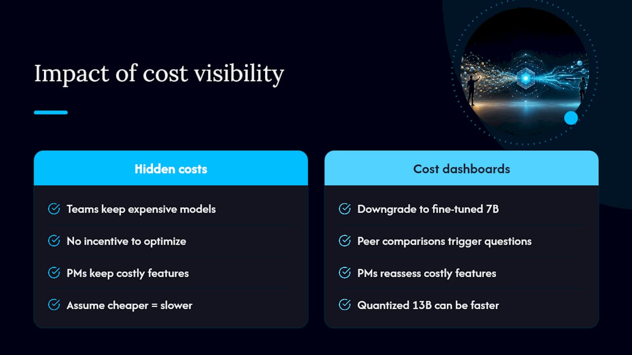
Every team that builds on top of an LLM fleet believes their use case justifies the expensive model. They’re usually wrong, but they have no incentive to find out because they don’t see the bill. The moment you give each team a cost dashboard showing their cost_per_outcome alongside their peers, the conversation changes. Engineers start asking whether they actually need GPT-4o for a task that a fine-tuned 7B model handles just as well. Product managers start questioning whether a feature that costs $0.40 per user interaction is worth keeping.
The second thing most playbooks miss: latency and cost are not always in tension. The assumption that cheaper models are slower is often wrong. A well-quantized 13B model running on dedicated hardware can outperform a frontier API call on latency while costing a fraction of the price. The real trade-off is accuracy on complex tasks, and the only way to know where that line sits for your specific workload is to run the experiment. Shadow testing is not optional — it’s the only honest way to make the routing decision.
On a platform like Theagentgames, where every agent inference call is a credit expenditure that directly affects a builder’s competitive budget, cost-aware engineering isn’t just an infrastructure concern. It’s a product feature. Builders who understand their agents’ token consumption and route intelligently have a structural advantage over those who don’t. The same logic applies to any enterprise running LLMs at scale: cost discipline is a competitive capability, not a cost-cutting exercise.
Sources
- LLM cost optimization: 7 strategies to cut inference spend (CloudZero)
- llm-budget (PyPI project page)
- compute-cfo (GitHub)